The back-and-forth method

This page provides documentation for the source code used in the paper A fast approach to optimal transport: The back-and-forth method.

The original code was written in C. A MATLAB wrapper is provided at https://github.com/Math-Jacobs/bfm.

Introduction

We are interested in the optimal transport problem

\[\frac 1 2 W_2(\mu,\nu)^2=\min_{T_{\#}\mu=\nu} \int_{\Omega} \frac 1 2 \lVert T(x)-x\rVert^2 \,\mu(x)dx,\]

on the unit square \(\Omega=[0,1]^2\). Here \(\mu\) and \(\nu\) are two densities on \(\Omega\), and \(\lVert x-y\rVert^2=(x_1-y_1)^2+(x_2-y_2)^2\).

The code solves the dual Kantorovich problem

\[\max_{\phi,\psi} \int_{\Omega} \phi(y)\,\nu(y)dy + \int_{\Omega} \psi(x)\,\mu(x)dx,\]

over functions \(\phi,\psi\colon\Omega\to\mathbb{R}\) satisfying the constraints

\[\phi(y)+\psi(x)\le \frac 1 2 \lVert x-y\rVert^2.\]

Python

The simplest way to use the Python code is to run this notebook on Google Colab.

The notebook is also available on the GitHub repository.

Alternatively, to install the Python bindings on your machine, first run in a terminal

git clone https://github.com/Math-Jacobs/bfm

and then install the Python bindings by running

pip install ./bfm/python

You may then directly run example.py.

MATLAB

Installation

Requirements: FFTW (download here), MATLAB.

Download the C MEX file w2.c here or by cloning the GitHub repository.

Compile it: in a MATLAB session run

mex -O CFLAGS="\$CFLAGS -std=c99" -lfftw3 -lm w2.c

This will produce a MEX w2 function that you can use in MATLAB. You may need to use flags -I and -L to link to the FFTW3 library, e.g. mex -O CFLAGS="$CFLAGS -std=c++11" w2.c -lfftw3 -I/usr/local/include. See this page for more information on how to compile MEX files.

Usage

In a MATLAB session, run the command

[phi, psi] = w2(mu, nu, numIters, sigma);

Input:

• mu and nu are two \(N\times M\) arrays of nonnegative values which sum up to the same value.

• numIters is the total number of iterations.

• sigma is the initial step size of the gradient ascent iterations.

Output:

• phi and psi are \(N\times M\) arrays corresponding to the Kantorovich potentials \(\phi\) and \(\psi\).

Example 1

Let us first compute the optimal transport between the characterstic function of a disk and its translate. We discretize the problem with ~1 million points (\(1024\times 1024\)).

n = 1024;

[x,y] = meshgrid(linspace(0.5/n, 1-0.5/n, n));

mu = zeros(n);
idx = (x-0.25).^2 + (y-0.25).^2 < 0.125^2;
mu(idx) = 1;
mu = mu * n^2/sum(mu(:));

nu = zeros(n);
idx = (x-0.75).^2 + (y-0.75).^2 < 0.125^2;
nu(idx) = 1;
nu = nu * n^2/sum(nu(:));

subplot(1,2,1)
imagesc(mu, 'x',[0,1], 'y',[0,1]);
title('Initial density')

subplot(1,2,2)
imagesc(nu, 'x',[0,1], 'y',[0,1]);
title('Final density')

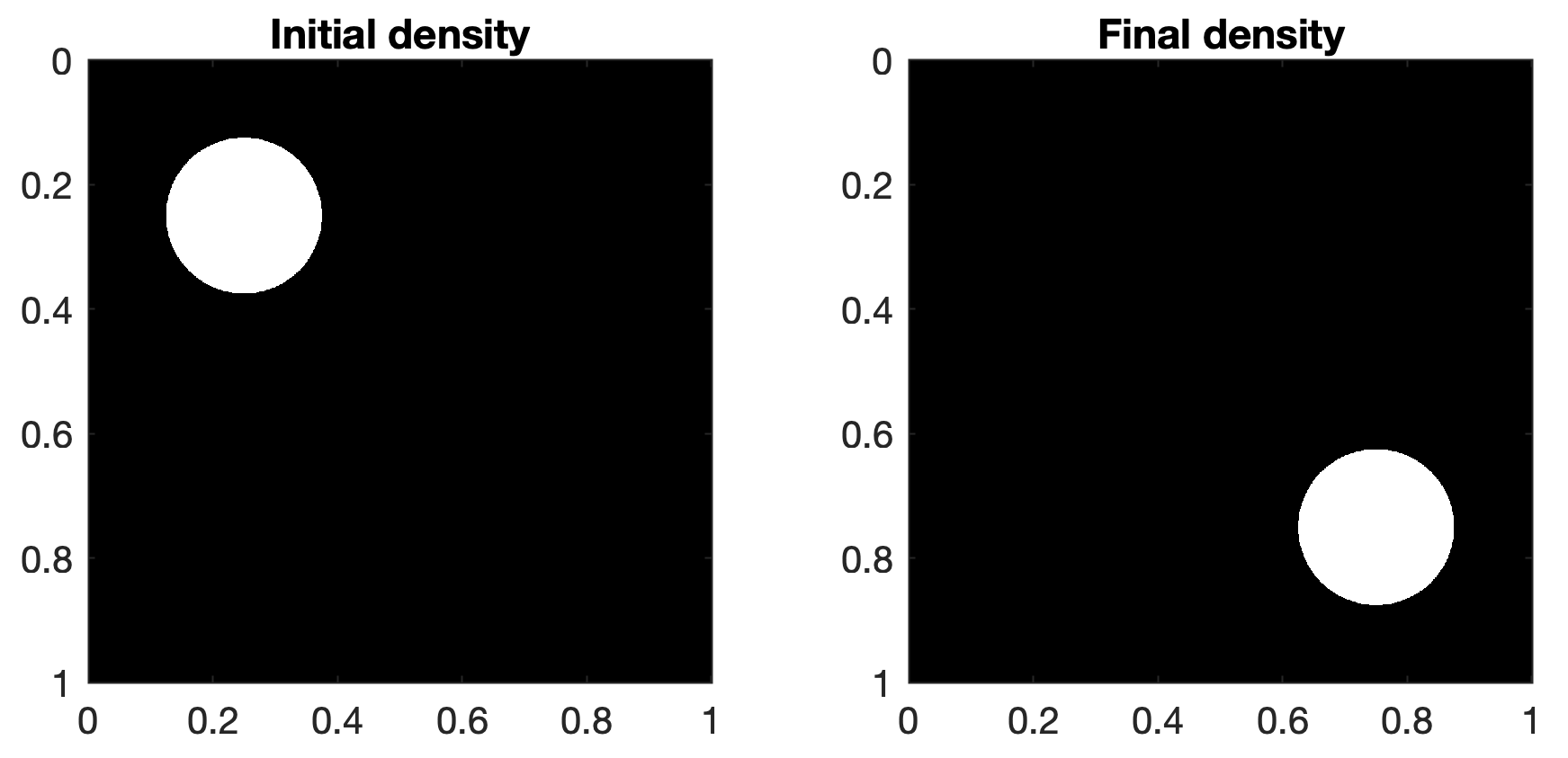
Here the densities are renormalized so that \(\int_\Omega\mu(x)dx=\int_\Omega\nu(x)dx=1\). Note that \(\nu\) is the translate of \(\mu\) by the vector \((\frac 1 2, \frac 1 2)\), and therefore \(\frac 1 2 W_2(\mu,\nu)^2=\frac 1 4\).

numIters = 10;
sigma = 8.0 / max(max(mu(:)), max(nu(:)));

tic;
[phi,psi] = w2(mu, nu, numIters, sigma);
toc

Output:

FFT setup time: 0.01s
iter  0, W2 value: 2.414694e-01
iter  5, W2 value: 2.500000e-01
iter 10, W2 value: 2.500000e-01
Elapsed time is 3.432973 seconds.

Example 2

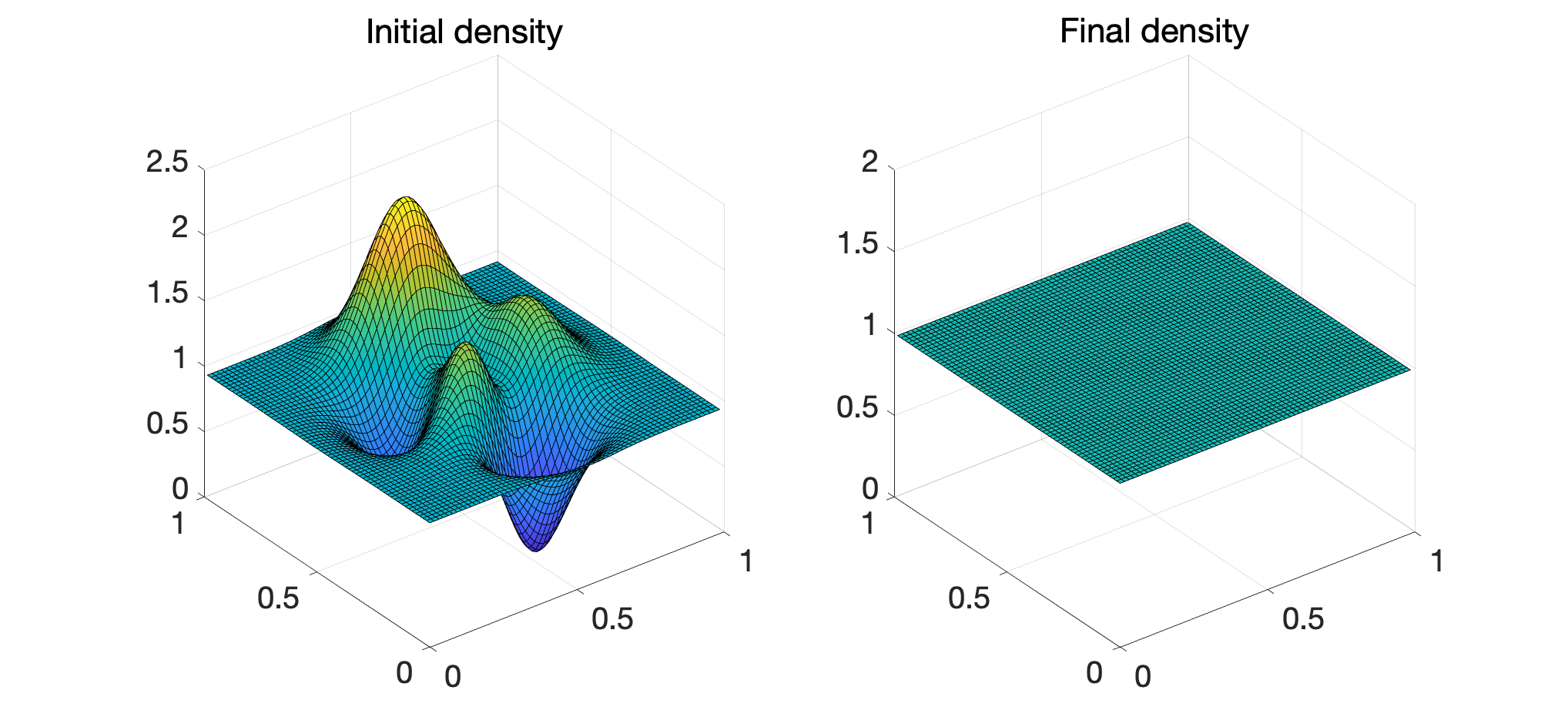
Let’s compute the optimal transport between the MATLAB peaks function and the uniform measure, on the 2d domain \([0,1]^2\).

We discretize the problem with ~1 million points (\(1024\times 1024\)) and plot the densities.

n = 1024;

[x,y] = meshgrid(linspace(0,1,n));

mu = peaks(n);
mu = mu - min(mu(:));
mu = mu * n^2/sum(mu(:));

nu = ones(n);

s = 16;         % plotting stride
subplot(1,2,1)
surf(x(1:s:end,1:s:end), y(1:s:end,1:s:end), mu(1:s:end,1:s:end))
title('Initial density')

subplot(1,2,2)
surf(x(1:s:end,1:s:end), y(1:s:end,1:s:end), nu(1:s:end,1:s:end))
title('Final density')

Then run the back-and-forth solver:

numIters = 20;
sigma = 8.0 / max(max(mu(:)), max(nu(:)));

tic;
[phi,psi] = w2(mu, nu, numIters, sigma);
toc

Output:

FFT setup time: 0.02s
iter  0, W2 value: -1.838164e-02
iter  5, W2 value: 9.791770e-04
iter 10, W2 value: 9.793307e-04
iter 15, W2 value: 9.793364e-04
iter 20, W2 value: 9.793362e-04
Elapsed time is 10.016858 seconds.

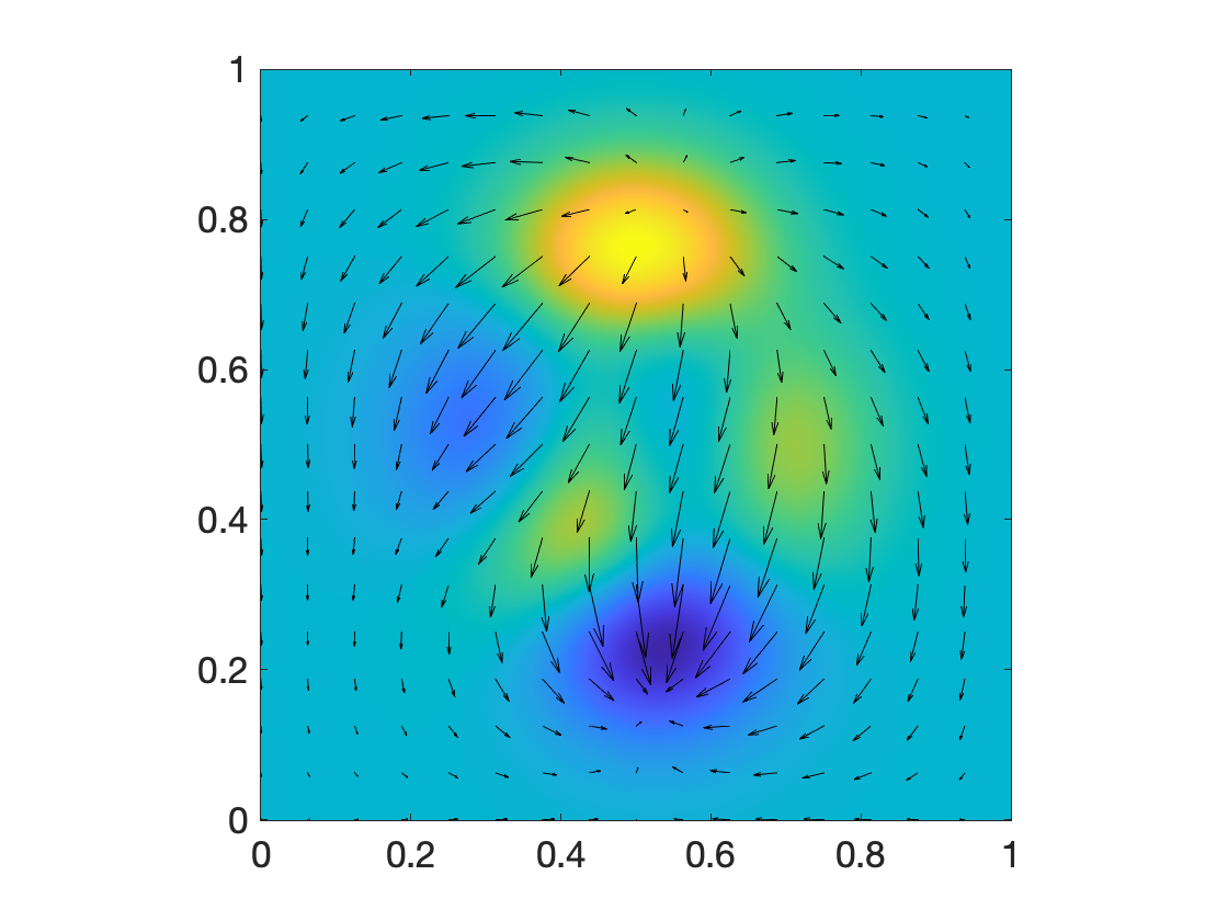
Finally compute the optimal transport map

\[T(x)=x-\nabla\psi(x)\]

and display the displacement \(m=-\nabla\psi\) as a vector field.

[mx, my] = gradient(-psi, 1/n);

figure;
imagesc(mu,'x',[0,1],'y',[0,1]);
axis square
set(gca,'YDir','normal')

hold on
s = 64;
quiver(x(1:s:end,1:s:end), y(1:s:end,1:s:end), ...
        mx(1:s:end,1:s:end), my(1:s:end,1:s:end), ...
         0, 'Color','k');

References

[1] Matt Jacobs and Flavien Léger. A fast approach to optimal transport: The back-and-forth method. Numerische Mathematik (2020): 1-32.